Chapter 6 Accessing Twitter’s API in R

Twitter is a unique source for data, for many reasons: along with text, it includes date and time information, and data on the type of device anr/or software used to post the tweet. What we often do not have reliable Twitter data on is location. There are two ways for Twitter to record your location: one is created during your Twitter account setup, where you (optionally) fill in where you are located. Many users fill in joke locations (The Milky Way, 3rd Rock From the Sun). To do something with location data, it’d have to be somewhat standardized, i.e. text inputs for Town and State.Without these prompts, values vary wildly, from ‘North Dakota’ to ‘Brooklyn’ to ‘27510,’ so it’s really not very useful data.

The other way Twitter will record your location is by geolocating your exact position. This has to be turned on or off, by choosing if Twitter can use your location on your device. Many users - most, in fact - have location services turned off. That means if you use geolocation data, you’re only observing data from users who have opted in to location services for twitter. That’s a subset of Twitter users that will drastically skew our results, so I also discourage its use.

One other caveat with Twitter, which can be frustrating to new users: you can’t go back in time and look at every Tweet ever posted. (Access to this is referred to as Twitter’s ‘Firehose.’) Just searching Twitter for a term will only return results from the last seven days. How can we get around this limitation?

One way is to analyze an individual account, or Twitter handle - this will allow us to download thousands of Tweets, assuming we’re looking at a prolific user.

The other way, which is beyond the scope of this Chapter, is to set up a loop in R that grabs Tweets every minute, or hour, or day, and records them, over time, to a database. This (obviously) requires pre-planning, so you can’t just do a lengthy report on the history and progression of the #MeToo movement on Twitter: you can only record the present and future. (Note that some interesting historical Twitter activity has been downloaded and shared online, such as the accounts of everyone in the Trump White House during his Presidency.)

Why is all of this so complicated? Well, Twitter’s valuation is based almost entirely on this huge collection of data it’s made (the Firehose), and granting access to historical Twitter data is one way Twitter actually makes money.

Like many proprietary online sources of data, Twitter gives data analysts this limited access to their real-time data via what’s called an API, or Application Programming Interface. That means instead of downloading every tweet ever made onto your laptop, you can use this ‘interface’ to access the database of information online and only grab the relevant data. Another example may help clarify: How could we analyze the headlines of the New York Times over the last 50 years? We cannot download all of that text onto our computer, of course, but the Times provides limited historical access via their API as well. Again, the limitations are somewhat severe, as they are protecting their intellectual property: The NY Times API only allows you to get ten results every minute. In other words, you query the API, get 10 results, wait a minute, and then you can get the next 10 results.

Note: One of our media analytics students Tyler Oldham made a package that automates this process \[here\] (‘https://github.com/toldham2/nytall’).

6.1 Making Your First Request to the New Twitter API v2

OK, so how do we gain access to an API? We’ll use Twitter as our example, as it’s overly complicated. But generally speaking, you need to have an account with the service. Twitter is free, and you need a Twitter account to access the API. (The New York Times is behind a paywall, but you can still create an account on their website and access the aPI for free without a subscription.)

So, first and foremost, create a Twitter account if you don’t have one (don’t worry, you never have to Tweet.)

Then, go to dev.twitter.com while signed in. Now, we are going to apply the v2 Twitter API. It includes several new features and improvements compared to the previous version, Twitter API v1.1. One of the most significant changes in Twitter API v2 is the introduction of a new set of modular endpoints, which allow developers to access specific sets of data and functionality more easily.

You can follow this link (https://developer.twitter.com/en/docs/tutorials/step-by-step-guide-to-making-your-first-request-to-the-twitter-api-v2) to see Step-by-step guide to making your first request to the new Twitter API v2.

At this time, there are three different levels of access that are applied at the Project-level:

Essential access: This access level is provided to anyone who has signed up for a developer account. (free) - Number of Apps within that Project: 1 - Tweet consumption cap: 500,000 Tweets per month

Elevated access: This access level is provided to anyone who has applied for additional access via the developer portal. (free) - Number of Apps within that Project: 3 - Tweet consumption cap: 2 million Tweets per month

Academic research access: This access level is provided to academic researchers who meet a certain set of requirements and applied for additional access via the developer portal. (need to apply) - Number of Apps within that Project: 1 - Tweet consumption cap: 10 million Tweets per month

6.2 Using You Twitter App in R

Start by installing the ‘rtweet’ package from CRAN:

install.packages('rtweet')

Once we’ve set up an App in the Twitter Developer Console, we need to connect our credentials to our R session.

First, we have to ‘tell’ Twitter who we are and what App we’re using, buy entering in our API Key and Secret. Let’s start by loading a package that will allow for authentication via a Web Browser:

## load rtweet
library(rtweet)

#more information on rtweet: https://cran.r-project.org/web/packages/rtweet/rtweet.pdf

Once our app is set up in dev.twitter.com, we should be able to generate four secret codes:

API Key (also known as consumer key)
API Secret (also known as consumer secret)
Access Token
Access Secret

All of these values can be generated from the ‘Keys and Tokens’ tab of your App’s page on dev.twitter.com.

Run this in R - be sure to replace “YOUR_APP_NAME” and “XXXXX” with the name of your App in the Twitter Developer Portal:

create_token(
app = "YOUR_APP_NAME_HERE",
consumer_key = "XXXXXXXXXXXXXXXXXXX",
consumer_secret = "XXXXXXXXXXXXXXXXXXX",
access_token = "XXXXXXXXXXXXXXXXXXX",
access_secret = "XXXXXXXXXXXXXXXXXXX",
set_renv = TRUE
) -> twitter_token

Let’s grab the last 3,000+ tweets from the Pope:

mytoken <- create_token(
  app = "MEA3290FALLTEACHING", #app name here
  consumer_key = "tKMrTovHc5WDej3skv50ydiBX", #consumer key here
  consumer_secret = "cuVLeICFGV82dyJaxL5wowmU6khsdIMPDZZJH6l0QpUaR16IKm", #consumer secret here
  access_token = "1942203541-j9vVz9wl3TinMD9JTzxW6SpkHt62zAE0lYune87", #access token here
  access_secret = "Cjaese8kXV3eVyGx9utFsX5khSzjYwzk1Jc0kpxvFBigs") #access secret here

pope <- get_timeline("pontifex", n = 18000, retryonratelimit = TRUE, token = mytoken)

If you don’t have any luck, you can download the version of the Pope’s tweets that I’m using in my analysis here:

library(downloadthis)

pope %>%
  download_this(
    output_name = "pope_tweets",
    output_extension = ".csv",
    button_label = "Download data",
    button_type = "default",
    self_contained = TRUE,
    has_icon = TRUE,
    icon = "fa fa-save",
    id = "pope-btn"
  )

You’ll also need to import it - if you copy it into your Project’s folder, you can simply run the command pope <- read.csv(file = 'pope_tweets.csv', header = FALSE)

6.3 Analyzing Twitter Data

OK, now we can use content from Twitter and analyze aspects such as:

Time, day and date of tweet frequency
Device(s) and App(s) used to Tweet
Lots of other metadata, like if each tweet was a retweet, or was flagged in certain counties, etc.

And of course we can collect all of the text from tweets and analyze them as we would a book.

Let’s start with time.

6.3.1 Lubridate & Working with Time

Lubridate is a really useful R package. You can ask it to break any collection of dates into days, weeks, months or years. And if it doesn’t recognize the format of your date column, you can ‘tell’ it how to read correctly. Let’s try using it on Twitter data.

install.packages('lubridate')

The ‘created_at’ column of our Twitter data contains our date information. Let’s try some things out:

library(tidyverse)

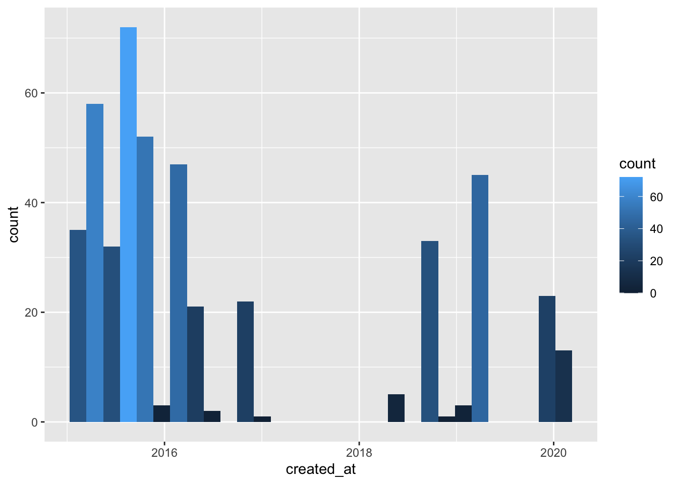
ggplot(pope, aes(x = created_at)) + geom_histogram(aes(fill = ..count..))

## `stat_bin()` using `bins = 30`. Pick better value with `binwidth`.

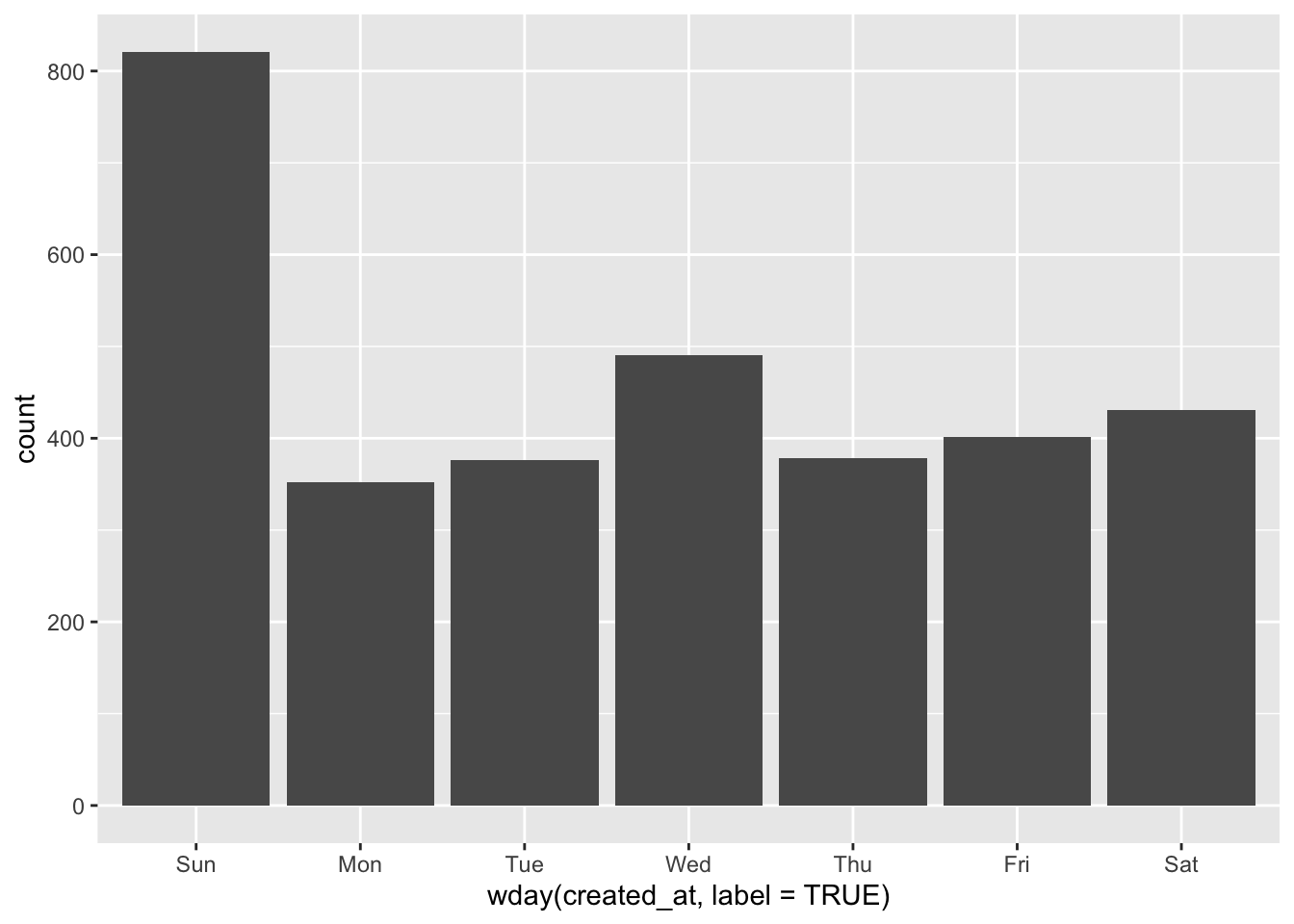
OK, we see the frequency over the past few years that the Pope has tweeted - but it’s pretty hard to understand. Let’s tweak it with a lubridate command to show the days of the week:

library(lubridate)
ggplot(pope, aes(x=wday(created_at, label = TRUE))) +
  geom_bar()

OK, that’s much clearer and makes a lot of sense!

6.3.2 Tweet Source

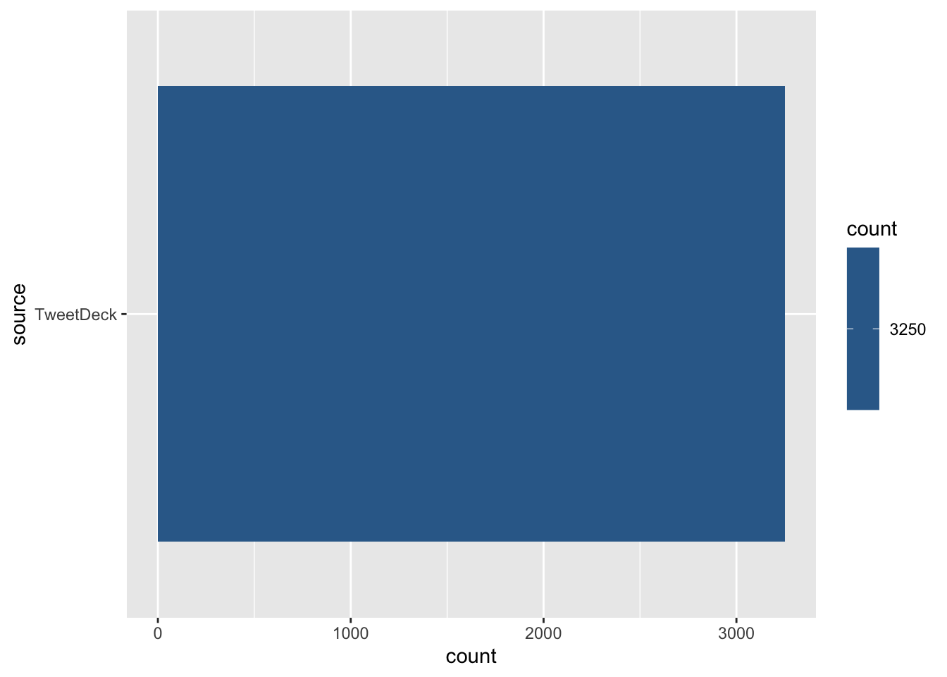
Did the user tweet from their phone? From a computer? Did they use a social media app that help them maintain consistency across platforms? Did an aide post it?

These are the questions we can answer by analyzing the source column of Twitter data:

ggplot(pope, aes(source)) + geom_bar(aes(fill = ..count..)) + coord_flip()

Wow, that’s boring. Let’s check if the President has a more varied source for tweets:

prez <- get_timeline('potus', n=18000, retryonratelimit = TRUE)

ggplot(prez, aes(source)) + geom_bar(aes(fill = ..count..)) + coord_flip()

A few notes about our plots:

We are using geom_bar() instead of geom_col() - they look the same, but geom_col() often requires extra parameters like ‘bin width.’
We earlier used geom_histogram. A histogram is like a line chart that ‘bins’ values into groups; think of plotting age: you wouldn’t have 90 or 100 lines to represent every age in your survey, you’d bin them: 0-10 years, 11-20 years, etc. Histograms visualize binned, continuous data.
The syntax of our ggplot’s is just weird. What’s up with ‘..count..?’ Why do we have two sets of aesthetics? Well, ..count.. is a special variables that can be used in ggplot - another is ..density.. . As for the separate aesthetics, the first set creates the bar chart based on the data values, and the second set colors the bars. We can control the aesthetics of those two calculations separately.

6.3.3 Text Analysis in Twitter

We can again use the tidytext package to create and analyze tokens:

library(tidytext)
pope %>% 
  unnest_tokens(word, text) %>% 
  anti_join(stop_words) %>% 
  count(word, sort = TRUE)

## Joining, by = "word"

## # A tibble: 8,997 × 2
##    word       n
##    <chr>  <int>
##  1 god      824
##  2 love     547
##  3 jesus    523
##  4 life     511
##  5 t.co     491
##  6 https    490
##  7 lord     490
##  8 peace    440
##  9 people   354
## 10 world    338
## # … with 8,987 more rows

That certainly looks correct, although there are a few words that don’t seem to make sense: t.co and https . t.co is short for twitter.com, and the https is part of a link, of course. You may also see amp, which is short for ampersand.

Let’s filter out these needless words:

pope %>% 
  unnest_tokens(word, text) %>% 
  anti_join(stop_words) %>% 
  filter(!word %in% c("https", "t.co")) %>% 
  count(word, sort = TRUE)

## Joining, by = "word"

## # A tibble: 8,995 × 2
##    word       n
##    <chr>  <int>
##  1 god      824
##  2 love     547
##  3 jesus    523
##  4 life     511
##  5 lord     490
##  6 peace    440
##  7 people   354
##  8 world    338
##  9 prayer   280
## 10 heart    256
## # … with 8,985 more rows

Cool. How about a word cloud?

library(wordcloud2)
# more about wordcloud2: https://r-graph-gallery.com/196-the-wordcloud2-library.html
pope %>% 
  unnest_tokens(word, text) %>% 
  anti_join(stop_words) %>% 
  filter(!word %in% c("https", "t.co")) %>% 
  count(word, sort = TRUE) %>% 
  wordcloud2()

## Joining, by = "word"

6.4 Search Keywords/Search Users by Keywords/Hashtags

tweets <- search_tweets(q = "chatgpt", n = 100,
                        lang = "en",
                        include_rts = FALSE)
# the max # of n is 18000

top_words <- tweets %>% 
  unnest_tokens(word, text) %>% 
  anti_join(stop_words) %>% 
  filter(!word %in% c("https", "t.co", "chatgpt", "gpt")) %>% 
  count(word, sort = TRUE) %>% 
  head(10)

## Joining, by = "word"

top_words %>% 
  ggplot(aes(reorder(word,n),n,fill = word)) +
  geom_col() +
  coord_flip()

More information of search tips

https://www.rdocumentation.org/packages/rtweet/versions/0.7.0/topics/search_tweets

users <- search_users("chatgpt", n = 100)

## Searching for users...

## Finished collecting users!

user_description <- users %>% 
  unnest_tokens(word, description) %>% 
  anti_join(stop_words) %>% 
  filter(!word %in% c("https", "t.co", "chatgpt", "gpt")) %>% 
  count(word, sort = TRUE) %>% 
  head(10)

## Joining, by = "word"

user_description %>% 
  ggplot(aes(reorder(word,n),n,fill = word)) +
  geom_col() +
  coord_flip()

6.5 Assignment

Learning Objectives

Get to know how to use Twitter APIs to collect tweets for a client/topic of your choice.

Step 1 Discuss with your group members to select a brand/person’s Twitter account that your group would like to collect data from.

Step 2 Collect the most recent 1000 tweets from your client’s Twitter account, as well as your client’s Twitter follower information.

step 3 Explore the Twitter data you collected to answer the questions below:

What’s the date range of the 1000 tweets you collected for your client?
How many of the 1000 tweets are retweets?
How many of the 1000 tweets are original? Among the original tweets, how many are messages sent to others?
Which original tweet has been retweeted most? Please describe this tweet.
Which original tweet has been favorited most? Please describe this tweet.
Among the 1000 tweets, how many have media URLs?
Among your client’s followers, which one has the greatest number of followers? What is that user’s most recent tweet/retweet? Also, describe the user’s profile.
Among your client’s followers, which one has been listed by other Twitter users most? What is that user’s most recent tweet/retweet? Also, describe the user’s profile.

Step 4 Discuss the implications of your answers and create a 5-7 mins presentation.

6.5.1 Sample code

create_token(
app = "YOUR_APP_NAME_HERE",
consumer_key = "XXXXXXXXXXXXXXXXXXX",
consumer_secret = "XXXXXXXXXXXXXXXXXXX",
access_token = "XXXXXXXXXXXXXXXXXXX",
access_secret = "XXXXXXXXXXXXXXXXXXX",
set_renv = TRUE
) -> mytoken

Collect owned twitter data through Twitter API

dt_timeline <- get_timelines("elonedge", n = 1000, token = mytoken) 
#The most recent 1000 tweets, question 1: click the dt_timeline in environment to see "created at" for date range.

ggplot(dt_timeline, aes(x = created_at)) + 
  geom_histogram(aes(fill = ..count..))

## `stat_bin()` using `bins = 30`. Pick better value with `binwidth`.

#Develop the visualization

Question 2 & 3 How many of the 1000 tweets are retweets/original? Among the original tweets, how many are messages sent to others?

dt_rt <- dt_timeline %>% 
  group_by(is_retweet) %>% 
  count(is_retweet)

dt_me <- dt_timeline %>% 
  filter(is_retweet=="FALSE") %>% 
  filter(!is.na(reply_to_screen_name)) %>% 
  count(is_retweet)

# Basic piechart
# Create Data
type <- data.frame(
  group=c("retweet", "orginial", "message"),
  value=c(81,381,6))
#change the value based on your own findings.

# Basic piechart
ggplot(type, aes(x="", y=value, fill=group)) +
  geom_bar(stat="identity", width=1, color="white") +
  coord_polar("y", start=0) +
  theme_void() # remove background, grid, numeric labels

Questions 4-6 Which original tweet has been retweeted most? Which original tweet has been favorited most? Among the 1000 tweets, how many have media URLs?

Toptweet_1 <- dt_timeline %>% 
  filter(retweet_count == max(retweet_count)) %>% 
  select(text,created_at,retweet_count)

Toptweet_2 <- dt_timeline %>% 
  filter(favorite_count == max(favorite_count)) %>% 
  select(text,created_at,favorite_count)

url <- dt_timeline %>% 
  filter(!is.na(media_url)) %>% 
  count(media_url)

Questions 7 & 8

Among your client’s followers, which one has the greatest number of followers? What is that user’s most recent tweet/retweet?

Among your client’s followers, which one has been listed by other Twitter users most? What is that user’s most recent tweet/retweet?

#Get the following and follower information

friends <- get_friends("elonedge") 
#get a user's friends

followers <- get_followers("elonedge") 
#get a user's followers

#Collect data from a user's friends/followers. 
bio_fr <-  lookup_users(friends$user_id[1:20]) 
bio_fr_full <-  lookup_users(friends$user_id) 

bio_fl <-  lookup_users(followers$user_id[1:20]) 
bio_fl_full <-  lookup_users(followers$user_id) 

#If you would like to save the follower id
#save_as_csv(bio_fl_full, "~/yourpath/elonedge_follower.csv") 

#Top follower
Topfollower_1 <- bio_fl_full %>% 
  filter(followers_count == max(followers_count)) %>% 
  select(text,created_at,location,description,followers_count)

Topfollower_2 <- bio_fl_full %>% 
  filter(listed_count == max(listed_count)) %>% 
  select(text,created_at,location,description,followers_count)